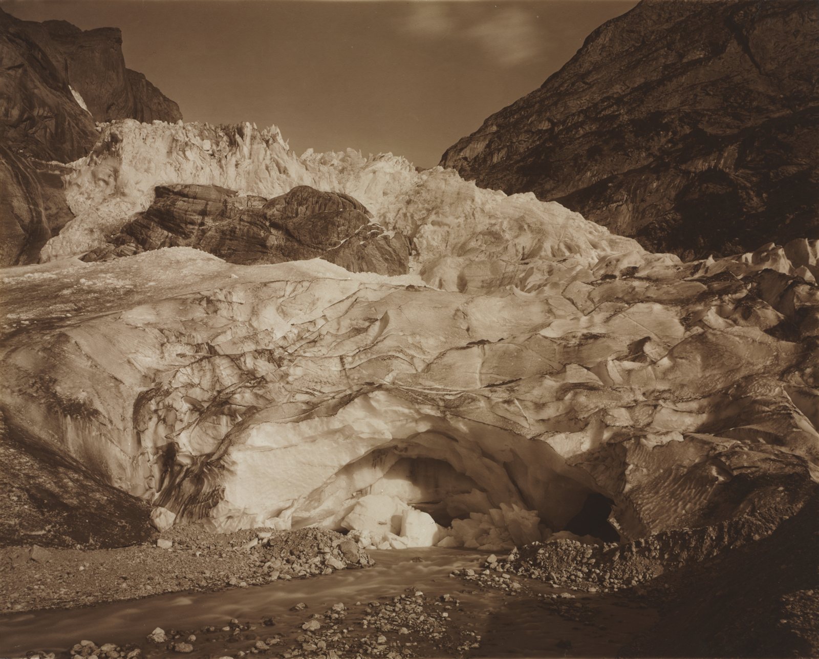
Erosion, ice and the shaping of landscapes

An old black-and-white photograph shows a tongue of ice between rocky mountains, and a river flowing out of it in the foreground. — The Upper Grindelwald Glacier, in Switzerland, from which the Lütschine river emerges: photograph by Adolphe Braun, around 1875–1877. Adolphe Braun, CC0, source

The idea that ice ages follow variations in the Earth’s orbit was set aside for decades: nobody knew how to test it.

Twice in this field, a correct idea had to wait for its instrument.

The first is continental drift, rejected for forty years because the ocean floor could not be observed. The second concerns the very origin of the great glacial cycles.

An explanation set aside

In the first half of the twentieth century, the mathematician and astrophysicist Milutin Milankovitch proposed an innovative explanation for the great glaciations: that they were driven by slow variations in the Earth’s orbit and axis.¹

The Earth does not always move in the same way. Its orbit stretches and becomes more circular again (eccentricity), the tilt of its axis varies (obliquity), and that axis wobbles like a spinning top (precession) — all on cycles of 20,000 to 100,000 years. These astronomical variations change the amount of sunlight received at high latitudes.

The hypothesis was set aside for several decades. Not because it seemed absurd, but because no one knew how to test it: that would have required a continuous record of climate over several hundred thousand years.

What changed

In the 1970s, researchers at last gained access to such a record: marine sediment cores, taken from the ocean floor. These stacks of deep-sea mud record, layer after layer and over millions of years, variations in temperature and in the volume of ice.²

A theory predicted rhythms, with figures attached. Researchers looked for them in the sediments. They were there.

What exactly was found

The 1976 paper does not say “we find the cycles”. It gives three peaks, and their share of the climate variations:³

a peak at around 23,000 years, which explains about 10% of the variations;
a peak at 42,000 years — about 25%;
a peak at 100,000 years — about 50%.⁴

One detail is decisive: the 42,000-year peak has exactly the period of the tilt of the Earth’s axis, and keeps a constant offset with it. It is not merely the right rhythm: it is the right rhythm, always in phase.⁵

This approach has the same rigour as the empty slots in Mendeleev’s periodic table: a number announced by theory, then verified in the field. It is what this site calls a risky prediction — had the astronomical frequencies not been found in the sediments, the hypothesis would have collapsed.

The authors’ own reservation

They do not conclude that everything is explained. They write that the 100,000-year cycle probably requires one more hypothesis: that the climate does not respond to it in simple proportion to what the orbit delivers.⁶

The anomaly is visible in the figures above: the 100,000-year cycle is the dominant one — and it is also the hardest to explain. According to the authors, one probably has to assume that the climate does not react in a simple, proportional way. Half a century later, this discrepancy has still not been fully resolved.

A confirmed theory is not a finished theory.

What is measured on glaciers, and how

A glacier is not a motionless mass: it accumulates snow at altitude and loses mass through melting lower down. What is measured is the balance of this mass, expressed in metres of water equivalent.⁷

The current rate runs to hundreds of billions of tonnes lost every year — around four hundred. For comparison, it was less than a hundred billion a year in 1976–1995, and around two hundred and thirty between 1996 and 2015.
Each recent year breaks or comes close to previous records. In the mid-2020s, the nineteen glacier regions of the world were all losing mass, several years in a row — a situation unprecedented in the records.
Of the roughly one hundred and sixty glaciers monitored in the field, almost all lose mass every year. The rare gains can be counted on the fingers of one hand.⁸

This page gives orders of magnitude rather than the balance for the most recent year, and this is deliberate: that balance changes every twelve months, whereas the rate and the direction do not.

Which is the worst year? It depends on the unit and on when the data are consulted. In tonnes, it is 2023. In metres of water equivalent, the sources contradict one another — some give 2023, others 2024 — because the WGMS recalculates its series as new measurements enter the database. This is not a flaw: it is what a living dataset does. But it means that a ranking must always be given with the date it was consulted.⁹

A dizzying figure

Since 1975, the cumulative loss from mountain glaciers has exceeded 9,000 billion tonnes of ice.¹⁰

But the most striking fact is the acceleration: 41% of this total loss recorded since 1976 occurred in the single decade 2015–2024.

Almost half of half a century’s melting was concentrated in ten years.

How errors are avoided

The method explains why these figures are robust.

Glaciers are not evenly distributed across the globe: some regions have tens of thousands of them, others very few. If one simply averaged all the glaciers measured, the most heavily instrumented areas would swamp the global average.

The scientific method works differently: an average value is first calculated for each region — nineteen regions in all — and these data are then combined. Each region is thus weighted according to its actual glacier area, not the number of sensors installed.¹¹

It is a safeguard against sampling bias, just as crucial as the measurement itself.

An apparent discrepancy resolved at last

Two official sources may give different values for cumulative glacier loss: more than 27 metres for one, more than 25 metres for the other.¹²

This is not a contradiction; three methodological choices need to be made explicit:

The starting year. The series do not begin at the same date (1950, 1960 or 1976). The further back one goes into the twentieth century, the higher the cumulative total.
The sample studied. The reference network comprises only around sixty glaciers monitored over the very long term. Conversely, recent space-based analyses observe almost all of the world’s glaciers by satellite.
The unit of measurement. “Thirty metres of ice” and “twenty-seven metres of water equivalent” denote the same quantity. Since ice is less dense than water (about 0.9), thirty metres of melted ice give exactly twenty-seven metres of water.¹³

The upshot

None of these figures is wrong, but none can be understood in isolation.

A glacier mass-balance measurement must always be stated with its reference year, its sample and its unit. These parameters are essential for any rigorous comparison of data.

What carves the valleys

Erosion does nothing spectacular in the short term. It is the work of running water, of frost that wears and splits rock, of wind and of the slow advance of ice.

The four tools, and the marks they leave

Each agent of erosion works in its own way, and each leaves a recognisable form. A geologist reads a landscape as one reads handwriting: the form reveals the tool.

Running water. A river cuts down into its bed and carries debris downstream. It produces V-shaped valleys, narrow at the bottom, because it attacks along a line. As it approaches the sea it slows down, can no longer carry its load, and deposits it: this is how deltas and alluvial plains form.
Ice. A glacier does not just flow, it planes. It acts across its whole width and tears away even the valley walls, producing U-shaped valleys, wide and flat-bottomed. Most often, it does not carve a new valley: it settles into the one a river had already cut into a V, and widens it. The two tools therefore work one after the other, in the same place, and the final form shows which one came last. The glacier pushes heaps of unsorted debris ahead of it and leaves them along its sides: the moraines — piles of stones of all sizes mixed together, which betray the passage of ice even tens of thousands of years later.
Frost. Water that seeps into a crack freezes, expands and splits the rock. Repeated every winter night, this mechanism is enough to break up a cliff and cover its foot with scree.
Wind. It carries only sand and dust, but it hurls them ceaselessly against the rocks. It shapes dunes, polishes surfaces, and undercuts rocks at the base — where the sand strikes hardest.¹⁴

These forms make it possible to read the past. A U-shaped valley in a region where there is no longer a glacier means that there once was one. This is how the extent of the ice of twenty thousand years ago was mapped, long before any direct measurement was available — and it is what made possible the debate described on this page.

In the heart of the Alps, erosion reaches about 0.1 to 1 millimetre a year. This rate is tens to hundreds of times slower than the growth of human fingernails (about 1 centimetre every three months); but, repeated over millions of years, this wear is enough to sculpt valleys several thousand metres deep.¹⁵

A writing rule: the scale of geological time

This field deals with durations that defy intuition. The words “rapid”, “abrupt” or “slow” should never be used without specifying the frame of reference.

An event described as “rapid” in geology can extend over 10,000 years. Conversely, a transformation spread over a century is a shock of extreme violence on the timescale of rocks.

Note 1

A century ago, Serbian scientist Milutin Milankovitch hypothesized the long-term, collective effects of changes in Earth's position relative to the Sun are a strong driver of Earth's long-term climate, and are responsible for triggering the beginning and end of glaciation periods (Ice Ages). […] The shape of Earth's orbit, known as eccentricity; The angle Earth's axis is tilted with respect to Earth's orbital plane, known as obliquity; and The direction Earth's axis of rotation is pointed, known as precession.

NASA Science Editorial Team, “Milankovitch (Orbital) Cycles and Their Role in Earth’s Climate”, NASA Science, 27 February 2020, updated 22 October 2024

Bibliography

12
- Bierman, Paul R. and Montgomery, David R., Key Concepts in Geomorphology, Macmillan Learning, 2020, in libraries (the agents of erosion and the forms they produce: V-shaped and U-shaped valleys, moraines, scree, dunes).
- Champagnac, Jean-Daniel et al., “Erosion-Driven Uplift of the Modern Central Alps”, Tectonophysics, vol. 474, 2009, p. 236-249, paywalled (Alpine erosion rates of the order of 0.1 to 1 mm/yr).
- Earle, Steven, Physical Geology, 2nd ed., BCcampus, 2019, sections 5.1 “Mechanical Weathering”, 13.4 “Stream Types”, 16.3 “Glacial Erosion” and 16.4 “Glacial Deposition”, open access (the V-shaped valleys of mountain streams, glacial erosion by rock fragments embedded in the ice, U-shaped valleys, moraines of unsorted sediment, talus slopes produced by frost). https://opentextbc.ca/physicalgeology2ed/chapter/16-3-glacial-erosion/
- Hays, James D., Imbrie, John and Shackleton, Nicholas J., “Variations in the Earth’s Orbit: Pacemaker of the Ice Ages”, Science, vol. 194, no. 4270, 1976, p. 1121-1132, paywalled (the three peaks at 100,000, 42,000 and 23,000 years and their respective shares of about 50, 25 and 10%; the constant phase relationship between the 42,000-year peak and obliquity; the authors’ reservation about the 100,000-year cycle, which implies a non-linear response of the climate). https://doi.org/10.1126/science.194.4270.1121
- Hugonnet, R. et al., “Accelerated Global Glacier Mass Loss in the Early Twenty-First Century”, Nature, vol. 592, no. 7856, 2021, p. 726-731, paywalled (elevation changes of all the Earth’s glaciers tracked using satellite archives). https://doi.org/10.1038/s41586-021-03436-z
- Milanković, Milutin, Kanon der Erdbestrahlung und seine Anwendung auf das Eiszeitenproblem, Académie royale serbe, Belgrade, 1941, in libraries (the astronomical theory of glaciations).